Introduction

Groundwater modeling has been started with the first computers in the 70ies and has been studied a lot in the last decades.
With the new potential of Cloud-Computing and quasi unlimited CPU-Resources available, the possibility of more exact prediction of the models is very high. On the other hand, the climate-change makes it necessary to involve real-time measurement and continuous calibration of the models, while physical parameters of soil and water quality a changing steadily.

The results of the inverse problem must are used to solve forward problems that answer the specific questions of the final users [2]

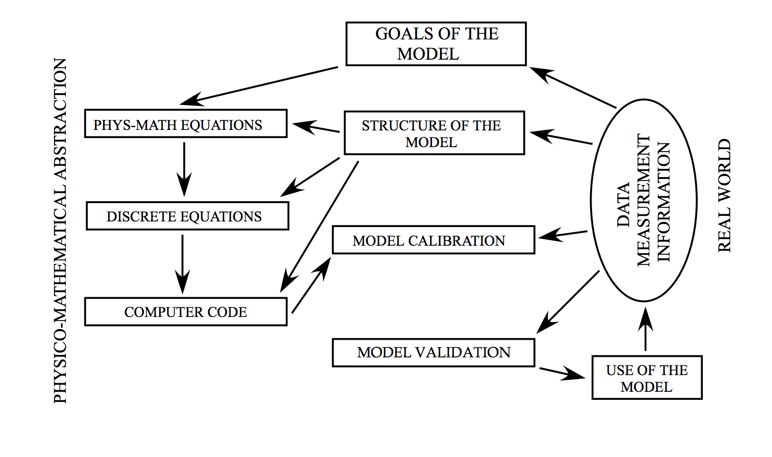
The development of a groundwater model or environmental models in general is shown in the next figure found in [3]:

Forward Problems vs. Inverse Problems

To build a model for a real groundwater system, two problems, the forward problem (simulation) and its inverse (calibration), must be solved. We must first solve the inverse problem to find appropriate model structure and model parameters, and then solve the forward problem to obtain required prediction results. Clearly, the model quality can not be improved by increasing only the accuracy of forward solutions if the inverse problem is not well solved. [1]

While forward models in groundwater modelling are very well developed, the progress of inverse solution techniques is blocked because of the following problems:

• ill-posed inverse problems with non-unique and unstable observation errors
• insufficient quantity and quality of observation data
• model structure errors

Forward Problems in Groundwater Modeling

Mathematical Models

A mathematical model is an equation or a set of equations which cas approximte an excitation-response relation of a system, based commonly on physical or experimental rules.

Example 1.1.1

The relationship between the well drawdown S and the pumping rate Q can be represented by the following equation:

$ S = aQ + bQ^2 $ (1.1.1)

where a and b are constant coefficients, depending on aquifer and well structure.
In this case, the pumping rate Q is the excitation and the drawdown S is the response.
a and b are describing the specific particularities of the system.

Example 1.1.2

The relationship between rainfall and a spring current in this area can be represented by a convolution integral:

$ g(t) = \int_0^t K(t-\tau) p(\tau) d\tau $ (1.1.2)

with:

• K (*): which characterizes the paricularities of the precipitation-spring system
• p(t): excitation at time t
• g(t): response at time t

Example 1.1.3

The average concentration C(t) of a given contaminant can be written as the Ordinary Differential Equation (ODE)

$ {d(VC) \over dt} = A (NC_N + RC_R - PC) $ (1.1.3)

with:

• V: volume of water in the aquifer ($L^3$)
• A: surface area of the aquifer ($L^3$)
• N: natural recharge rate for unit area of aquifer ($L/T$)
• R: artificial recharge rate for unit area of aquifer ($L/T$)
• P: pumping rate for unit area of aquifer ($L/T$)
• CN: average concentration in natural recharge water ($M/L^3$)
• CR: average concentration of artificial recharge water ($M/L^3$)

To determine a solution for this equation, an initial condition $C(0) = C_0$ must be given. The function will be integrated mathematically and on every integration a constant c has to be added. With the initial concentration, the integration constant will be determined.

So, the model consists of an ODE and an initial condition.

• state variable: C(t) (concentration) as the response
• control variables: P, R and CN can be seen as the excitation
• parameters: V, A, N and CR

Example 1.1.4

Two-dimensional groundwater flow in an isotropic and confined aquifer is governed by a partial differential equation (PDE)

$ S {\delta \phi \over \delta t} = \nabla \bullet (T \nabla \phi)-Q$, $ (x,y) \in (\Omega) $, $ t \geq 0 $ (1.1.4)

initial and boundary conditions:

• $ \phi(x, y, t)|_{t=0} = f_0(x,y) $,
• $ \phi(x, y, t)|_{(\Gamma _1)} = f_1(x,y,t) $,
• $ T \nabla \phi \bullet n|_{(\Gamma _2)} = f_2(x,y,t)$,

where:

• $ \phi(x, y, t) $: piezometric head ($ L $)
• $ S(x, y) $: storage coefficient ($-$)
• $ T(x, y) $: transmissivity ($ L^2/T $)
• $ Q(x, y, t) $: sink/source term ($ L/T $)
• $ \nabla = (\delta/\delta x, \delta/\delta y) $: the gradient operator vector
• $ (\Omega) $: flow region in horizontal plan $ (x, y) $ with boundary sections $ (\Gamma_1) $ and $ (\Gamma_2) $
• $ n $: unit normal vector of $ (\Gamma_2) $
• $ f_1, f_2, f_3 $: given functions
• $ x, y $: horizontal coordinates $ (L) $
• $ t $: time $ (T) $

The parameters here are:

• state variable: $ \phi $ as the response
• control variable: $ Q $ as the control variable (excitation)
• system parameters: $ T $ and $ S $

References

[1]: “Inverse Problems in Groundwater Modeling”
[2]: “Giudici M. 2003. Inverse Modelling for Flow and Transport in Porous Media”
[3]: “Giudici M. 2001. Development, calibration and validation of physical models, in Geographic Information Systems and Environmental Modeling (K. C. Clarke, B. O. Parks and M. C. Krane, Eds.), 100-121, Prentice-Hall, Upper Saddle River (NJ).”